A gearbox bearing that fails after nine months is rarely the result of bad arithmetic. Bearing life calculation is a short formula, but the number it produces depends on inputs that come from the machine rather than from the catalogue: the equivalent dynamic load, the real operating speed, the lubrication film and the contamination level.
The answer, stated up front, is that basic rating life follows L10 = (C / P)^p, where C is the dynamic load rating, P is the equivalent dynamic load, and p is 3 for ball bearings and 10/3 for roller bearings. Because the load ratio is raised to a power, the result is far more sensitive to P than to anything else in the equation. Moving the load ratio from 0.10 to 0.12 removes roughly 42 percent of the calculated life, and no premium grease will give it back.
What follows covers the formula itself, the adjustment factors that turn a theoretical L10 into a number you can plan maintenance around, four visual comparisons of loads, conditions and bearing types, and a short checklist to run before you commit to a service interval.
The Basic Formula and a Worked Example
The basic rating life L10 is the life that 90 percent of an identical group of bearings reaches or exceeds before the first sign of material fatigue. It is normally expressed in millions of revolutions, which converts to hours once the speed is known.
L10 = (C / P)^p, in millions of revolutions. L10h = (1,000,000 / (60 n)) multiplied by (C / P)^p, in operating hours, where n is the speed in revolutions per minute.
Take a small deep groove ball bearing with a dynamic capacity C of 14 kN, an equivalent load P of 1.4 kN and a shaft speed of 1,500 rpm. The load ratio is 0.10, so L10 equals 1,000 million revolutions and L10h equals about 11,111 hours, which is roughly fifteen months of continuous running. Raise the real load to 1.68 kN and the ratio becomes 0.12, so the same bearing gives about 6,400 hours. Nothing else changed.
The formula assumes a fully developed lubrication film, correct fitting, no misalignment and no wear from contamination or stray current. Each of those assumptions has to be checked separately, because the basic rating life treats them as ideal conditions.
Why the Load Ratio Dominates the Result
Life is proportional to the load ratio raised to the power p, so a change in load is amplified in the result. Doubling the load cuts the life of a ball bearing to one eighth of its value, and the same doubling cuts a roller bearing to about one tenth. The shape of that relationship is easier to read from a chart than from a table of numbers.
Basic rating life against load ratio
The curve shows the basic rating life in hours at 1,500 rpm, plotted against the load ratio from 0.05 to 0.30. The vertical axis is logarithmic, so each grid line represents a tenfold change rather than a fixed step. Dropping the load ratio from 0.05 to 0.10 on its own costs a factor of eight in life, from 88,889 hours to 11,111 hours. Between 0.20 and 0.30 the curve looks flatter on this scale, yet the values still fall from 1,389 hours to 411 hours. The practical point is that the first few percent of extra load costs far more life than the last few percent, which is why load measurement deserves more attention than the arithmetic.
Equivalent Dynamic Load: Where Most Calculations Go Wrong
P is not the radial load you read from the drawing unless the bearing carries pure radial load with a rotating inner ring. When radial and axial forces act together, P = X times Fr plus Y times Fa, and the factors X and Y come from the bearing data sheet.
For deep groove ball bearings, the ratio of axial to radial load against the value e, typically between 0.22 and 0.44, decides whether the axial term is included at all. Angular contact bearings use Y values in the range of 1.0 to 2.2. A modest axial force from a helical gear, a vertical pump or a misaligned coupling can therefore add 30 to 60 percent to the effective load, and the cubic exponent turns that into a much shorter life.
Forces that never appear on the layout drawing matter just as much: belt pull, unbalanced masses, chain tension and the extra load created by an interference fit that consumes internal clearance. A short conversation with the mechanical designer is cheaper than a failed calculation.
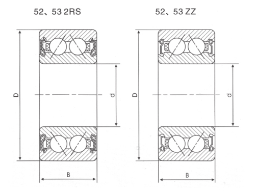
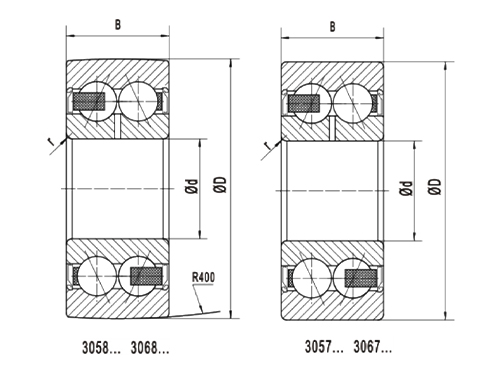
Where combined loads are unavoidable and space is tight, a double row angular contact design carries radial and axial forces in one unit, which simplifies both the bearing arrangement and the load case you have to describe in the calculation.
Clearance, Preload and Temperature Change the Load You Assumed
A preloaded bearing enters service with a constant axial load already applied, and in lightly loaded positions that preload can be the largest single component of P. Preload raises stiffness and lowers noise, but it has to be chosen against the life target, so it helps to understand how preload and clearance change the operating load before a value is fixed.
Temperature works from the other direction. A shaft running 40 degrees warmer than its housing grows relative to the housing, and if the internal clearance is small the bearing becomes axially pinched. The same mechanism appears in ordinary motor applications, where the temperature rise is enough to consume clearance and shift the contact angle, as described in this note on thermal expansion of deep groove ball bearings.
Both effects push the real load above the value used on paper, so treat the calculation as a check on a design decision rather than a replacement for one.
Adjusted Rating Life: Reliability, Lubrication and Material
Few applications can accept a 10 percent failure probability. The modified rating life multiplies the basic value by adjustment factors: Lnm = a1 multiplied by aISO multiplied by L10. The reliability factor a1 falls sharply as the target rises.
Reliability factors applied to a base life of 8,000 hours at 1,500 rpm
Required reliability
Failure probability
a1 factor
Resulting L10h
90 percent
10 percent
1.00
8,000 h
95 percent
5 percent
0.64
5,120 h
96 percent
4 percent
0.55
4,400 h
97 percent
3 percent
0.47
3,760 h
98 percent
2 percent
0.37
2,960 h
99 percent
1 percent
0.25
2,000 h
The operating condition factor aISO produces the widest spread of all. In a machine with clean oil and a thick lubricant film the factor can exceed 1.5, while a boundary film with water ingress can push it below 0.3. The bars below show what that spread means in hours for a bearing with a clean base life of 8,000 hours.
Adjusted life under different operating conditions
Sealed bearing, clean oil, full film
13,600 h
Normal industrial cleanliness
8,000 h
Slight contamination or water ingress
4,400 h
Heavy contamination, boundary film
2,000 h
Starved lubrication, thin film
1,200 h
All five bars start from the same 8,000 hour base life and apply a different operating condition factor. A sealed bearing running in clean oil reaches 13,600 hours, while the same bearing in a heavily contaminated housing falls to 2,000 hours. The gap between the top and the bottom bar is more than eleven times the life, produced by lubrication and contamination alone. No load has changed in this comparison, and the dynamic capacity C is identical in every case. The largest single gain therefore comes from protecting the bearing rather than from ordering a bigger one.
Ball or Roller: Choosing the Right Exponent
The exponent differs because the contact geometry differs. Ball bearings use p = 3, roller bearings use p = 10/3, and that fractional exponent is the main reason a roller bearing often shows a longer calculated life at the same load ratio. The comparison below keeps the envelope and the speed identical so that only the exponent changes.
Ball bearing versus roller bearing at three load ratios
The chart compares a ball bearing and a roller bearing of similar envelope at three load ratios, all at 1,500 rpm. At a load ratio of 0.10 the roller bearing reaches about 23,900 hours against 11,111 hours for the ball bearing. The absolute gap narrows as the load rises, but the roller bearing keeps an advantage of roughly 1.7 to 2.2 times across the range shown. That advantage comes from applying an exponent of 10/3 instead of 3 to the same load ratio. Roller bearings also bring higher friction and a greater sensitivity to misalignment, so the extra hours are not free.
Varying Loads and Speeds: The Duty Cycle Method
Most machines do not run at one load and one speed for their whole life. Divide the working cycle into conditions, estimate the time share q of each one, and combine them into a single equivalent load.
At constant speed, the equivalent load is the cubic mean: Pm equals the cube root of the sum of q multiplied by P cubed, using the exponent 10/3 for roller bearings instead of 3. When the speed also changes, calculate L10h for each condition and then combine the results: the total life is the reciprocal of the sum of the time fractions divided by their individual lives.
A duty cycle calculation also shows which part of the cycle deserves attention. It is common for 20 percent of the operating time to consume most of the calculated life, and that condition is where a small change in load or alignment pays back fastest.
Roller elements are often used for the heavily loaded part of a duty cycle, because the higher exponent rewards their greater load capacity when the peak condition dominates the total damage.
Comparing Bearing Types Before You Calculate
The formula ranks bearings of a given type accurately, but it does not tell you which type to use in the first place. Where a machine needs axial capacity in both directions inside a compact envelope, double row angular contact bearings are the usual answer, and their axial factors make them competitive once the combined load is described correctly.
Six properties that shape the life number
The radar compares two common arrangements on six properties that influence the life number you eventually type into the calculation. The single row deep groove ball bearing scores well on noise, misalignment tolerance and cost, but gives up axial capacity. The double row angular contact ball bearing carries more radial and axial load in the same envelope, and its higher stiffness usually supports a longer calculated life at the same load ratio. Misalignment tolerance is its weak point, because both rows share the load and a tilted housing concentrates stress on one row. Use a chart like this to shortlist a type, then calculate L10 separately for each shortlisted option.
A Short Checklist Before You Sign Off the Number
Use a measured or calculated load, and include belt pull, gear forces and the effect of fits.
Take C from the manufacturer data for the exact variant, including seals and clearance class.
Confirm that the speed used in the hours conversion is the real operating speed, not the nameplate speed.
Check that the lubrication method can build a film at the lowest expected speed and temperature.
Set the reliability target and apply a1 before comparing quotations from different suppliers.
Recalculate the duty cycle with the worst condition included, not only with the nominal one.
File the calculation with the machine record so the next inspection can be compared with the prediction.
Bearing life calculation is not a marketing exercise; it is a way to test an assumption before metal is cut. The formula takes two lines, but the quality of the answer depends on the load you measured, the speed you verified and the lubrication you can actually maintain.
A number that matches reality is worth more than a number that looks impressive on a datasheet. Run the calculation for the worst condition in the duty cycle, compare two shortlisted types on the same basis, and keep the result beside the maintenance record. When the next bearing comes out of that machine, you will know within minutes whether the calculation or the application was wrong.